R or Python for machine learning. Creating a Machine Learning Classifier Using Scikit-learn in Python

Development of categorization applications RSS feeds using Python, NLTK and machine learning

Getting to know Python

This article is intended for software developers—especially those with experience in Ruby or Java—who are new to machine learning.

Challenge: Using machine learning to categorize RSS feeds

I was recently tasked with creating an RSS feed categorization system for a client. The task was to read dozens and even hundreds of messages in RSS feeds and automatically assign them to one of dozens of predefined topics. The daily output of this categorization and news feed system would influence the content, navigation, and search capabilities of the client's website.

The customer representative suggested using machine learning, possibly based on Apache Mahout and Hadoop, as she had recently read about these technologies. However, the developers on both her team and ours had more experience with Ruby than with Java™. In this article, I talk about all the technical research, the learning process and, finally, the final implementation of the solution.

What is machine learning?

My first question in this project was: “What is machine learning really?” I heard this term and knew that IBM supercomputer® Watson recently beat real people at the game Jeopardy. As an online shopper and social media user, I also realized that Amazon.com and Facebook do a great job of tailoring recommendations (products or people) based on data about their customers. In short, machine learning lies at the intersection of IT, mathematics and natural language. This process mainly involves the following three aspects, but the solution for our client was based on the first two:

• Classification. Assigning elements to pre-declared categories based on training data for similar elements.
• Recommendation. Selecting recommended elements based on observations of the selection of similar elements
• Clustering. Identifying subgroups in a data set

Failed attempt - Mahout and Ruby

Having understood what machine learning is, we moved on to the next step - finding ways to implement it. The client suggested that Mahout might be a good starting point. I downloaded the code from Apache server and started learning the machine learning process in Mahout and Hadoop. Unfortunately, I found Mahout to be difficult to learn even for an experienced Java developer and lacking working code examples. No less upsetting limited quantity infrastructures and gem packages for machine learning in Ruby.

Nakhodka - Python and NLTK

I continued searching for a solution; Python was consistently found in search results. As a Ruby devotee, I knew that Python was a dynamic programming language and used the same object-oriented text-based interpretation model, although I had never studied the language. Despite these similarities, I shied away from learning Python for many years, considering it unnecessary knowledge. So Python was my blind spot, and I suspect it's the same for many fellow Ruby programmers.

A search for books on machine learning and a detailed study of their contents showed that a significant part of such systems are implemented in Python in combination with the Natural Language Toolkit (NLTK) library for working with natural languages. Further research revealed that Python is used much more often than I thought, for example in the Google App engine, on YouTube, and on websites using Django. It turns out that it comes natively installed on the Mac OS X workstations that I work with every day! Moreover, Python has interesting standard libraries (for example, NumPy and SciPy) for mathematical calculations, scientific research and engineering solutions. Who could have known?

After discovering some elegant code examples, I decided to use a Python solution. For example, the one-line code below does everything needed to receive an RSS feed by HTTP protocol and print its contents:

print feedparser.parse("http://feeds.nytimes.com/nyt/rss/Technology")

Moving towards the goal with Python

When learning a new programming language, the easiest part is learning the language itself. A more complex process is studying the ecosystem. You need to figure out how to install it, how to add libraries, write code, structure files, run, debug and prepare tests. In this part we present brief introduction to these sections; Don't forget to look through the links in the section - there may be a lot of useful information there.

pip

Python Package Index (pip) is the standard package manager in Python. This is the program you will use to add libraries to your system. It is similar to gem for Ruby libraries. To add the NLTK library to your system, you need to run the following command:

$ pip install nltk

To display a list of Python libraries installed on your system, use the command:

$pip freeze

Launching programs

Running Python programs is just as easy. If you have a program locomotive_main.py that takes three arguments, you can compile and run the code using the following python command:

$ python locomotive_main.py arg1 arg2 arg3

The if __name__ == "__main__" syntax given in is used in Python to determine whether a file is running separately from command line or caused by another piece of code. To make a program executable, add a check for "__main__" to it.

Listing 1. Checking Main status

import sys import time import locomotive if __name__ == "__main__": start_time = time.time() if len(sys.argv) > 1: app = locomotive.app.Application() ... additional logic...

virtualenv

Many Ruby programmers are familiar with the problem of shared system libraries, also called gems. Using system-wide library sets is generally undesirable because one of your projects may rely on version 1.0.0 of an existing library and another on version 1.2.7. Java developers face a similar problem with the system-wide CLASSPATH variable. Similar to the rvm tool in Ruby, Python uses the virtualenv tool (see link in section ) to create separate program execution environments, including special Python instructions and library sets. The commands in show how to create a virtual runtime named p1_env for your p1 project, which will include the feedparser, numpy, scipy, and nltk libraries.

Listing 2. Creation virtual environment execution with virtualenv

$ sudo pip install virtualenv $ cd ~ $ mkdir p1 $ cd p1 $ virtualenv p1_env --distribute $ source p1_env/bin/activate (p1_env)[~/p1]$ pip install feedparser (p1_env)[~/p1]$ pip install numpy (p1_env)[~/p1]$ pip install scipy (p1_env)[~/p1]$ pip install nltk (p1_env)[~/p1]$ pip freeze

The script to activate your virtual environment must be run every time you work with your project in a shell window. Please note that after executing the activation script, the shell prompt changes. To make it easier to navigate to your project directory and activate the virtual environment after creating a shell window on your system, it is helpful to add an entry like the following to your ~/.bash_profile file:

$ alias p1="cd ~/p1 ; source p1_env/bin/activate"

Basic Code Structure

Having mastered simple "Hello World" level programs, a Python developer needs to learn how to properly structure code using directories and file names. Like Java or Ruby, Python has its own rules for this. In short, Python uses the concept of grouping related code together packages and uses uniquely defined namespaces. For demonstration purposes, this article places the code in the project's root directory, such as ~/p1. It contains a locomotive subdirectory containing the Python package of the same name. This directory structure is shown in.

Listing 3. Example directory structure

locomotive_main.py locomotive_tests.py locomotive/ __init__.py app.py capture.py category_associations.py classify.py news.py recommend.py rss.py locomotive_tests/ __init__.py app_test.py category_associations_test.py feed_item_test.pyc rss_item_test.py

Pay attention to the strangely named files __init__.py . These files contain Python instructions for loading the necessary libraries into your environment, as well as your custom applications, which are located in the same directory. The contents of the locomotive/__init__.py file are shown.

Listing 4. locomotive/__init__.py

# import system components; loading installed components import codecs import locale import sys # import application components; loading custom files *.py import app import capture import category_associations import classify import rss import news import recommend

With the locomotive package structure shown in , host programs in your project's root directory can import and use it. For example, the locomotive_main.py file contains following commands import:

import sys # >-- system library import time # >-- system library import locomotive # >-- user application code library # from the "locomotive" directory

Testing

The standard Python library unittest provides convenient testing resources. Java developers familiar with JUnit, as well as Ruby experts working with the Test::Unit framework, will easily understand the Python unittest code from .

Listing 5. Python unittest

class AppTest(unittest.TestCase): def setUp(self): self.app = locomotive.app.Application() def tearDown(self): pass def test_development_feeds_list(self): feeds_list = self.app.development_feeds_list() self.assertTrue (len(feeds_list) == 15) self.assertTrue("feed://news.yahoo.com/rss/stock-markets" in feeds_list)

The content also demonstrates distinctive feature Python: Code must be consistently indented to compile successfully. The tearDown(self) method may seem strange - why would a successful pass result be programmed into the test code? There's really nothing wrong with that. This way you can program an empty method in Python.

Tools

What I really needed was an integrated development environment (IDE) with syntax highlighting, code completion, and breakpoint execution to get the hang of Python. As a user of the Eclipse IDE for Java, the first thing I noticed was pyeclipse. This module works quite well, but sometimes it is very slow. In the end, I chose the PyCharm IDE, which met all my requirements.

So, armed with a basic knowledge of Python and its ecosystem, I was finally ready to implement machine learning.

Implementing categories in Python and NLTK

To build the solution, I needed to process simulated RSS news feeds, analyze their text using NaiveBayesClassifier, and then classify them into categories using the kNN algorithm. Each of these actions is described in this article.

Extracting and processing news feeds

One of the challenges of the project was that the client had not yet defined a list of target RSS news feeds. There was also no “training data.” Therefore, news feeds and training data had to be imitated at the initial stage of development.

The first method I used to obtain sample news feed data was to save the contents of a list of RSS feeds to a text file. Python has a very good library for parsing RSS feeds called feedparser, which allows you to hide the differences between various formats RSS and Atom. Another useful library for serializing simple text objects playfully named pickle (“pickle”). Both libraries are used in the code from , which saves each RSS feed in a "pickled" form for later use. As you can see, the Python code is concise and powerful.

Listing 6. CaptureFeeds class

import feedparser import pickle class CaptureFeeds: def __init__(self): for (i, url) in enumerate(self.rss_feeds_list()): self.capture_as_pickled_feed(url.strip(), i) def rss_feeds_list(self): f = open ("feeds_list.txt", "r") list = f.readlines() f.close return list def capture_as_pickled_feed(self, url, feed_index): feed = feedparser.parse(url) f = open("data/feed_" + str(feed_index) + ".pkl", "w") pickle.dump(feed, f) f.close() if __name__ == "__main__": cf = CaptureFeeds()

The next step turned out to be unexpectedly time-consuming. After receiving a sample of the tape data, I needed to categorize it for later use as training data. Training data is precisely the set of information that you provide to your categorization algorithm as a learning resource.

For example, one of the sample feeds I used was the ESPN sports news channel. One of the reports was that Tim Tebow of the Denver Broncos had been acquired by the New York Jets, and at the same time, the Broncos had signed Peyton Manning to become their new quarterback. Another message concerned Boeing and its new jet airliner. The question arises: into what category should the first story be classified? Great words include tebow, broncos, manning, jets, quarterback, trade, and nfl. But to indicate the category of training data, you only need to select one word. The same can be said about the second story - what to choose, Boeing or jet? The whole complexity of the work lay precisely in these details. Careful manual categorization of large amounts of training data is essential if you want your algorithm to produce accurate results. And the time that will have to be spent on this cannot be underestimated.

It soon became obvious that I needed more data to work, and it should already be divided into categories - and quite accurately. Where to look for such data? And this is where Python NLTK comes into the picture. In addition to the fact that this is an excellent library for processing texts in natural languages, it comes with ready-made downloadable sets of source data, the so-called. "cases", as well as software interfaces for easy access to this data. To install the Reuters corpus, you need to run the below commands and it will download over 10,000 news items in your ~/nltk_data/corpora/reuters/ directory. Like RSS feed elements, every Reuters news article contains a headline and a body, so NLTK's categorized data is ideal for emulating RSS news feeds.

$ python # enter the interactive Python shell >>> import nltk # import the nltk library >>> nltk.download() # launch the NLTK loader and enter "d" Identifier> reuters # specify the case "reuters"

Of particular interest is the file ~/nltk_data/corpora/reuters/cats.txt. It contains a list of file names with notes, as well as the categories assigned to each of the files. The following entries indicate that file 14828 in the test subdirectory is assigned to the grain theme.

test/14826 trade test/14828 grain

Natural language is hard

The raw material for our algorithm for categorizing RSS materials is, of course, simple texts on English language. The term “raw materials” is quite appropriate here.

English, like any other natural language (the language of everyday communication), is characterized by extreme heterogeneity and inconsistency from the point of view of computer processing. The first issue that arises is the register. Is it possible to count a word Bronco equal bronco? The answer will be: “possibly.” Punctuation and spacing are also important. Is it possible to compare bronco. With bronco or bronco,? Seems Yes. Then there are plural forms and similar words. Is it possible to count run, running And ran equivalent forms? Depends on the situation. These three words are the same root. What if words from natural language are also accompanied by HTML tags? In this case you will have to work with elements like bronco. Finally, there is the problem of frequently used but actually meaningless words such as articles, conjunctions and prepositions. These so-called filler words make processing more difficult. Thus, natural language is quite messy and requires cleaning up before it can be used.

Luckily, Python and NLTK make it easy for you to get rid of this junk. The normalized_words method from the RssItem class eliminates all these obstacles. In particular, notice how NLTK strips the raw text of an article of inline HTML tags with just one line of code! In addition, a regular expression removes punctuation, after which the text is divided into words and converted to lowercase.

Listing 7. RssItem class

class RssItem: ... regex = re.compile("[%s]" % re.escape(string.punctuation)) ... def normalized_words(self, article_text): words = oneline = article_text.replace("\n ", " ") cleaned = nltk.clean_html(oneline.strip()) toks1 = cleaned.split() for t1 in toks1: translated = self.regex.sub("", t1) toks2 = translated.split() for t2 in toks2: t2s = t2.strip().lower() if self.stop_words.has_key(t2s): pass else: words.append(t2s) return words

The list of auxiliary words is taken from NLTK with one command; Other natural languages ​​are also supported.

nltk.corpus.stopwords.words("english")

NLTK also provides several morphological analysis classes to further normalize words. You can learn more about morphological analysis, lemmatization, sentence structure analysis, and grammar in the NLTK documentation.

Naive Bayes classification

The Naive Bayes algorithm (naive Bayes algorithm) is widely known and is built into NLTK as the nltk.NaiveBayesClassifier class. The Bayesian algorithm allows you to classify elements based on the presence or absence of certain elements in their composition. In the case of RSS feeds, specific (purified) natural language words are used as elements. The algorithm is “simple” in the sense that it does not imply relationships between elements (in our case, words).

However, there are more than 250,000 words in the English language. I certainly wouldn't want to create an object with 250,000 boolean values ​​for each RSS feed to implement the algorithm. So what words to use? In short, these should be the most frequently occurring words in the test data that are not filler words. NLTK has a very handy class nltk.probability.FreqDist that allows you to identify these popular words. And the collect_all_words method given in , returns an array containing all the words from all training notes.

This array is then processed by the identify_top_words method, which returns the most frequently occurring words. Convenient feature The nltk.FreqDist class actually creates a hash, but its keys are sorted according to their corresponding values ​​(number of occurrences). This way, you can easily highlight the top 1000 most frequently occurring words by specifying the index range [:1000] as per Python syntax.

Listing 8. Using the nltk.FreqDist class

def collect_all_words(self, items): all_words = for item in items: for w in item.all_words: words.append(w) return all_words def identify_top_words(self, all_words): freq_dist = nltk.FreqDist(w.lower() for w in all_words) return freq_dist.keys()[:1000]

To simulate NLTK database RSS feeds from Reuters articles, I needed to create categories for each of them. I did this by reading the ~/nltk_data/corpora/reuters/cats.txt file that I mentioned earlier. Reading a file in Python is simple:

def read_reuters_metadata(self, cats_file): f = open(cats_file, "r") lines = f.readlines() f.close() return lines

The next step is to obtain the characteristics of each message from the RSS feed. This action is performed by the features method from the RssItem class, demonstrated below. When working this method the array of all words (all_words) of an article is first reduced to a smaller set of unique words (set) by eliminating duplicate words. Next, it goes through the list of the most common words top_words and checks their presence or absence in the article. As a result, we get a hash of 1000 logical values, the keys of which are the words themselves with the w_ prefix. The corresponding Python code is quite short.

def features(self, top_words): word_set = set(self.all_words) features = () for w in top_words: features["w_%s" % w] = (w in word_set) return features

Next, I collect a training set of RSS messages and their individual characteristics and pass them on to the algorithm for processing. The code from demonstrates the implementation of this task. Please note that training the classifier takes exactly one line of code.

Listing 9. Training nltk.NaiveBayesClassifier

def classify_reuters(self): ... training_set = for item in rss_items: features = item.features(top_words) tup = (features, item.category) # tup is a 2-element tuple featuresets.append(tup) classifier = nltk .NaiveBayesClassifier.train(training_set)

So, the NaiveBayesClassifier classifier, located in the memory of the running Python program, has been trained. Now I can simply go through the list of RSS feeds that need to be categorized and use the classifier to determine the category for each item. Very simple.

for item in rss_items_to_classify: features = item.features(top_words) category = classifier.classify(feat)

Less simple classification

As mentioned earlier, our algorithm does not imply the existence of relationships between individual parameters. Thus, phrases like "machine learning" and "learning machine" or "New York Jet" and "jet to New York" are equivalent (the preposition "to" is excluded as an auxiliary word). In natural language, there are obvious connections between these words. How can we make the algorithm less “simple” and teach it to recognize these relationships between words?

One method is to include common phrases of two ( bigrams) and three words ( trigrams). And we are no longer surprised that NLTK has support for these features in the form of the nltk.bigrams(...) and nltk.trigrams(...) functions. Just as the library selected the most common N words from the entire dataset, it can identify the most popular two- and three-word phrases and use them as parameters.

Your results may vary

Cleaning data and applying an algorithm is a bit of an art. Should we normalize the set of words even more, for example, by highlighting the roots? Or do you need to include more than 1000 of the most common words? Or less? Or maybe you need to use a larger training dataset? Or define more words as auxiliaries? You can ask all these questions to yourself. Experiment with them, try them, go through the mistakes, and you will be able to create the best algorithm for your data. I decided for myself that 85% is a good level of successful categorization.

The client wanted to display RSS feed items in a selected category or related categories. Now that the data had been categorized using a simple Bayes algorithm, the first part of the customer's requirements was fulfilled. The task of defining “related categories” turned out to be more difficult. In this case, you need to use recommendation systems based on machine learning algorithms. The recommendation system is based on the similarity of some elements to others. Good examples These features include product recommendations on Amazon.com and friend recommendations on Facebook.

The most popular algorithm for making recommendations is the k-Nearest Neighbors (kNN, k nearest neighbors) algorithm. The idea is to create a list of labels (categories) and associate each label with a set of data. Next, the algorithm compares the data sets, identifying matching elements. A data set is represented by a set of numerical values, usually normalized from 0 to 1. Similar labels can then be extracted based on the data sets. Unlike the naive Bayes algorithm, which produces one result, kNN can produce a whole list of recommendations with degrees of agreement (determined by the value of k).

I found the recommendation algorithms easier to understand and implement than the classification algorithms, although the code itself was longer and too mathematically complex to include here. Code examples for kNN can be found in Manning's excellent new book, Machine Learning in Action (see link in section). In our case of processing RSS feeds, the tag values ​​were the same as the categories, and the data sets were arrays of values ​​for the top 1000 most popular words. Once again, creating such an array is part science, part mathematics, and part art. For each word in the array, the value can be a Boolean value (0 or 1), a percentage frequency of the word, an exponential expression of frequency, or some other quantity.

Conclusion

Getting to know Python, NLTK and machine learning was interesting and enjoyable. Python is a powerful and concise programming language that has now become a core part of my developer toolkit. It is great for implementing machine learning, natural language processing, and math and science applications. Also, although I didn't mention it in this article, I found it useful for creating charts and graphs. And if Python has also been in your blind spot, I encourage you to get acquainted with it.

Hi all!

In this article I will talk about a new comfortable way to program in Python.

This is less like programming and more like creating articles (reports/demonstrations/research/examples): you can insert regular explanatory text among blocks of Python code. The result of executing the code is not only numbers and text (as is the case with the console when working with Python), but also graphs, diagrams, pictures...

Examples of documents you can create:

Looks cool? Do you want to create the same documents? Then this article is for you!

First you need to install the Anaconda package. What it is? This is a fully configured Python along with a pre-installed set of the most popular modules. Anaconda also includes the JupyterLab environment, in which we will create documents with Python code.

If you already have Python installed, uninstall it first. This can be done through the Programs and Features panel in the Control Panel.

Download

Download Anaconda for Python 3.6 (Windows 7 and above) or Python 2.7 (Windows XP).

The installation file weighs 500+ MB, so it can take quite a long time to download.

Installation

Run the downloaded file. The installer window will open. On the first two pages, immediately click “Next”. Next, you can choose to install Anaconda only for current user computer, or for everyone.

Important! In the next window you need to specify the path where Anaconda will be installed. Choose a path that does not contain folders with spaces in the name (for example, Program Files) and does not contain non-English Unicode characters (for example, Russian letters)!

Ignoring these rules can lead to problems when working with different modules!

Personally, I created an Anaconda folder right at the root of the C drive and specified the following path:

There will be two checkmarks on the last window. Leave everything as it is.

Finally, the installation will begin. It may take ~10 minutes. You can calmly drink tea :)

Anaconda Navigator

After successfully installing Anaconda, launch the Anaconda Navigator program from the Start menu. When you launch you should see this logo:

Then the navigator itself will open. This is the starting point for working with Anaconda.

In the central part of the window there are various programs, which are included in the Anaconda package. Some of them have already been installed.

We will mainly use “jupyterlab”: it is in it that beautiful documents are created.

The left side shows the navigator sections. By default, the “Home” section is open. In the “Environments” section, you can enable/disable/load additional Python modules using a convenient interface.

JupyterLab

In the “Home” section of the navigator, launch (the “Launch” button) the “jupyterlab” program (the very first one in the list).

Your default browser should open with the JupyterLab environment in a separate tab.

The contents of the folder C:\Users\ are displayed on the left<ИМЯ_ВАШЕЙ_УЧЕТНОЙ_ЗАПИСИ> .

The notepad file “untitled.ipynb” is open on the right. If there's nothing to the right, you can create a new, empty notebook by clicking on the "+" in the top left corner and selecting "Notebook Python 3":

Notebook

It's time to figure out what notebooks are.

Typically we write Python code in .py files, and then the Python interpreter executes them and outputs the data to the console. To conveniently work with such files, programming environments (IDEs) are often used. These include PyCharm, which I talked about in the article.

But there is another approach. It consists of creating notebooks with the ipynb extension. Notepads consist of a large number of blocks. There are blocks with in plain text, and there are blocks with Python code.

Try entering some Python code into the first block in the notepad. For example, I create a variable equal to the sum of the numbers 3 and 2:

On the next line we simply write the name of this variable. For what? You'll see now.

Now you need to execute this block. To do this, click on the triangle icon in the toolbar above the notepad or the Ctrl + Enter key combination:

Under the block with Python code, another block has appeared, which contains the output of the results of the previous block. Now the output contains the number 5. This number is output by the second line of the block we wrote.

In conventional programming environments, to achieve this effect we would have to write print(a) , but here we can omit the call to this function and simply write the name of the variable we want to print.

But you can display the values ​​(numbers and text) of variables (even through a function) in other programming environments.

Let's try to do something more complicated. For example, display some picture.

Create a new block using the button in the toolbar above the notepad.

In this block we download the Anaconda logo from the Wikimedia website and display it:

From PIL import Image import requests image_url = "https://upload.wikimedia.org/wikipedia/en/c/cd/Anaconda_Logo.png" im = Image.open(requests.get(image_url, stream=True).raw) im

The result will look like this:

This is something that conventional development environments are not capable of. And in JupyterLab - easily!

Now let's try to add a block with plain text between two already created blocks with Python code. To do this, select the first block by clicking and add a new block using the button in the toolbar. The new block will be inserted immediately after the first block.

If you did everything correctly, the result will look like this:

By default, blocks in JupyterLab are for Python code. In order to turn them into text blocks, you need to change their type through the toolbar. At the very end of the panel, open the list and select “Markdown”:

The selected block will turn into a block of text. The typed text can be formatted italics or make it bold. You can find more information on Markdown (text formatting tools).

This is how you can design text blocks in a notepad:

Export

In JupyterLab you can export your notebook to the most different formats. To do this, at the very top of the environment, select the “Notebook” tab. In the menu that opens, select “Export to...” and select the format (for example, PDF) into which you want to convert your notepad.

Here is a link to the gist with the notepad from this article.

Managing Python Modules

You can enable/disable/download modules from Anaconda Navigator. To do this, select “Environments” in the left menu:

By default, a list is displayed installed modules(~217 pieces). Among them are such popular ones as numpy (working with arrays) or scypi (scientific and engineering calculations).

To install new packages, in the drop-down menu above the table (where it says “Installed”), select “Not installed”:

The list will be updated - the list of uninstalled modules will be automatically loaded.

Check the boxes next to the modules you want to download, and then click on the “Apply” button in the lower right corner to download and install them. Once the process is complete, you will be able to use these modules in notebooks.

conclusions

You can concentrate on writing the algorithm and immediately visualizing the results of executing the code, instead of fiddling with complex programming environments for large programs and a console that can only output numbers and text.

Alexander Krot, a student at FIVT MIPT, my good friend and, recently, colleague, launched a series of articles about practical tools for intelligent analysis of big data and machine learning ( Data mining and machine learning).

3 articles have already been published, I hope there will be more in the future:
1) Introduction to Machine Learning with Python and Scikit-Learn
2) The Art of Feature Engineering in Machine Learning
3) When there is really a lot of data: Vowpal Wabbit

The published articles focus on the practical aspects of working with tools for automatic data analysis and with algorithms that allow you to prepare data for effective machine analysis. In particular, examples of code in Python are given (by the way, we recently started using Python) with the specialized library Scikit-Learn, which you can quickly run on your home computer or personal cloud to get a taste of big data yourself.

Recently I was thinking about how. Familiarity with the above tools will now allow you to conduct practical experiments in this direction (a Python program, by the way, can also be run on the Linux built into the controller, but a mobile processor is unlikely to handle examples of grinding gigabytes of data). And by the way, Scala is also respected among engineers working with big data; integrating such code will be even easier.

Traditionally, mastery of any tools does not eliminate the need to find a good problem that can be effectively solved with their help (unless, of course, someone else sets this task for you). But it opens up space for additional possibilities. In my opinion, it might look something like this: a robot (or a group of robots) collects information from sensors, sends it to a server, where it is accumulated and processed to look for patterns; Next, the algorithm will compare the found patterns with the operational values ​​of the robot’s sensors and send it predictions about the most likely behavior of the environment. Or, on the server, a knowledge base about the terrain or a certain type of terrain is prepared in advance (for example, in the form of characteristic photographs of the landscape and typical objects), and the robot will be able to use this knowledge to plan behavior in an operational environment.

I’ll steal the first article as a primer, the rest from the links on Habré:

Import numpy as np import urllib # url with dataset url = "http://archive.ics.uci.edu/ml/machine-learning-databases/pima-indians-diabetes/pima-indians-diabetes.data"# download the file raw_data = urllib.urlopen(url) # load the CSV file as a numpy matrix dataset = np.loadtxt(raw_data, delimiter="," ) # separate the data from the target attributes X = dataset[:,0 :7 ] y = dataset[:,8 ]

Data Normalization

Everyone is well aware that most gradient methods (on which almost all machine learning algorithms are essentially based) are very sensitive to data scaling. Therefore, before running algorithms, it is most often done either normalization, or the so-called standardization. Normalization involves replacing nominal features so that each of them lies in the range from 0 to 1. Standardization implies such data preprocessing, after which each feature has a mean of 0 and a variance of 1. Scikit-Learn already has functions ready for this:

From sklearn import preprocessing # normalize the data attributes normalized_X = preprocessing.normalize(X) # standardize the data attributes standardized_X = preprocessing.scale(X)

Feature selection

It is no secret that often the most important thing when solving a problem is the ability to correctly select and even create features. In English literature this is called Feature Selection And Feature Engineering. While Future Engineering is quite a creative process and relies more on intuition and expert knowledge, Feature Selection already has a large number of ready-made algorithms. “Tree” algorithms allow for calculating the information content of features:

From sklearn import metrics from sklearn.ensemble import ExtraTreesClassifier model = ExtraTreesClassifier() model.fit(X, y) # display the relative importance of each attribute print(model.feature_importances_)

All other methods are in one way or another based on efficient enumeration of subsets of features in order to find the best subset on which the constructed model gives the best quality. One such brute force algorithm is the Recursive Feature Elimination algorithm, which is also available in the Scikit-Learn library:

From sklearn.feature_selection import RFE from sklearn.linear_model import LogisticRegression model = LogisticRegression() # create the RFE model and select 3 attributes rfe = RFE(model, 3 ) rfe = rfe.fit(X, y) # summarize the selection of the attributes print(rfe.support_) print(rfe.ranking_)

Construction of the algorithm

As already noted, Scikit-Learn implements all the main machine learning algorithms. Let's look at some of them.

Logistic regression

It is most often used to solve classification problems (binary), but multi-class classification is also allowed (the so-called one-vs-all method). The advantage of this algorithm is that at the output for each object we have the probability of belonging to the class

From sklearn import metrics from sklearn.linear_model import LogisticRegression model = LogisticRegression() model.fit(X, y) print(model) # make predictions expected = y predicted = model.predict(X)

Naive Bayes

It is also one of the most famous machine learning algorithms, the main task of which is to restore the distribution densities of the training sample data. Often this method gives good quality in multi-class classification problems.

From sklearn import metrics from sklearn.naive_bayes import GaussianNB model = GaussianNB() model.fit(X, y) print(model) # make predictions expected = y predicted = model.predict(X) # summarize the fit of the model print(metrics.classification_report(expected, predicted)) print(metrics.confusion_matrix(expected, predicted))

K-nearest neighbors

Method kNN (k-Nearest Neighbors) often used as component more complex classification algorithm. For example, its assessment can be used as a sign for an object. And sometimes, a simple kNN on well-chosen features gives excellent quality. With proper settings of parameters (mainly metrics), the algorithm often gives good quality in regression problems

From sklearn import metrics from sklearn.neighbors import KNeighborsClassifier # fit a k-nearest neighbor model to the data model = KNeighborsClassifier() model.fit(X, y) print(model) # make predictions expected = y predicted = model.predict(X) # summarize the fit of the model print(metrics.classification_report(expected, predicted)) print(metrics.confusion_matrix(expected, predicted))

Decision trees

Classification and Regression Trees (CART) often used in problems in which objects have categorical characteristics and is used for regression and classification problems. Trees are very suitable for multi-class classification

From sklearn import metrics from sklearn.tree import DecisionTreeClassifier # fit a CART model to the data model = DecisionTreeClassifier() model.fit(X, y) print(model) # make predictions expected = y predicted = model.predict(X) # summarize the fit of the model print(metrics.classification_report(expected, predicted)) print(metrics.confusion_matrix(expected, predicted))

Support Vector Machine

SVM (Support Vector Machines) is one of the most famous machine learning algorithms, mainly used for classification task. Just like logistic regression, SVM allows multi-class classification using the one-vs-all method.

From sklearn import metrics from sklearn.svm import SVC # fit a SVM model to the data model = SVC() model.fit(X, y) print(model) # make predictions expected = y predicted = model.predict(X) # summarize the fit of the model print(metrics.classification_report(expected, predicted)) print(metrics.confusion_matrix(expected, predicted))

In addition to classification and regression algorithms, Scikit-Learn has great amount more complex algorithms, including clustering, as well as implemented techniques for constructing compositions of algorithms, including Bagging And Boosting.

Optimization of algorithm parameters

One of the most difficult steps in building truly effective algorithms is choosing the right parameters. Usually, this becomes easier with experience, but one way or another you have to go overboard. Fortunately, Scikit-Learn already has quite a few functions implemented for this purpose.

For example, let’s look at the selection of a regularization parameter, in which we take turns trying out several values:

Import numpy as np from sklearn.linear_model import Ridge from sklearn.grid_search import GridSearchCV # prepare a range of alpha values ​​to test alphas = np.array() # create and fit a ridge regression model, testing each alpha model = Ridge() grid = GridSearchCV(estimator=model, param_grid=dict(alpha=alphas)) grid.fit(X, y) print(grid) # summarize the results of the grid search print(grid.best_score_) print(grid.best_estimator_.alpha)

Sometimes it turns out to be more effective to randomly select a parameter from a given segment many times and measure the quality of the algorithm at this parameter and thus choose the best one:

Import numpy as np from scipy.stats import uniform as sp_rand from sklearn.linear_model import Ridge from sklearn.grid_search import RandomizedSearchCV # prepare a uniform distribution to sample for the alpha parameter param_grid = ("alpha" : sp_rand()) # create and fit a ridge regression model, testing random alpha values model = Ridge() rsearch = RandomizedSearchCV(estimator=model, param_distributions=param_grid, n_iter=100 ) rsearch.fit(X, y) print(rsearch) # summarize the results of the random parameter search print(rsearch.best_score_) print(rsearch.best_estimator_.alpha)

We have looked at the entire process of working with the Scikit-Learn library, with the exception of outputting the results back to a file, which is offered to the reader as an exercise, because one of the advantages of Python (and the Scikit-Learn library itself) compared to R is its excellent documentation. In the following parts we will consider in detail each of the sections, in particular, we will touch on such an important thing as Beauty Engineering.

I really hope that this material will help beginning Data Scientists start solving machine learning problems in practice as soon as possible. In conclusion, I would like to wish success and patience to those who are just starting to participate in machine learning competitions!

Python is a great programming language to implement for a variety of reasons. Firstly, Python has a clear syntax. Secondly, in Python It is very easy to manipulate text. Python use big number people and organizations all over the world, so it is evolving and well documented. The language is cross-platform and can be used completely free of charge.

Executable pseudo code

Intuitive syntax Python often called executable pseudo-code. Installation Python by default already includes high-level data types such as lists, tuples, dictionaries, sets, sequences, and so on, which the user no longer needs to implement. These high-level data types make it easy to implement abstract concepts. Python allows you to program in any style familiar to you: object-oriented, procedural, functional, and so on.

IN Python Text is easy to process and manipulate, making it ideal for processing non-numeric data. There are a number of libraries to use Python to access web pages, and intuitive text manipulation makes it easy to retrieve data from HTML-code.

Python popular

Programming language Python popular and the many code examples available make learning it easy and fairly quick. Secondly, popularity means that there are many modules available for different applications.

Python is a popular programming language in scientific as well as financial circles. A number of libraries for scientific computing such as SciPy And NumPy allow you to perform operations on vectors and matrices. It also makes the code even more readable and allows you to write code that looks like linear algebra expressions. In addition, scientific libraries SciPy And NumPy compiled using languages low level (WITH And Fortran), which makes calculations when using these tools much faster.

Scientific instruments Python work great in conjunction with a graphical tool called Matplotlib. Matplotlib can produce 2D and 3D plots and can handle most types of plots commonly used in the scientific community.

Python It also has an interactive shell that allows you to view and check elements of the program being developed.

New module Python, under the name Pylab, strives to combine opportunities NumPy, SciPy, And Matplotlib in one environment and installation. Today's package Pylab It is still under development, but it has a great future.

Advantages and disadvantages Python

People use different programming languages. But for many, a programming language is simply a tool for solving a problem. Python is a language top level, which allows you to spend more time understanding the data and less time thinking about how they should be presented to the computer.

The only real drawback Python is that it does not execute program code as quickly as, for example, Java or C. The reason for this is that Python- interpreted language. However, it is possible to call compiled C-programs from Python. This allows you to use the best of various languages programming and develop the program step by step. If you've experimented with an idea using Python and decided that this is exactly what you want to be implemented in the finished system, then this transition from prototype to work program. If the program is built on a modular basis, then you can first make sure that what you need works in the code written in Python, and then, to improve the speed of code execution, rewrite critical sections in the language C. Library C++ Boost makes this easy to do. Other tools such as Cython And PyPy allow you to increase program performance compared to normal Python.

If the idea itself being implemented by the program is “bad,” then it is better to understand this by spending a minimum of precious time writing code. If the idea works, then you can always improve performance by rewriting partially critical sections of the program code.

In recent years, a large number of developers, including those with advanced degrees, have worked to improve the performance of the language and its individual packages. Therefore, it is not a fact that you will write code in C, which will work faster than what is already available in Python.

Which version of Python should I use?

Nowadays, different versions of this are in common use at the same time, namely 2.x and 3.x. The third version is still under active development, most of the various libraries are guaranteed to work on the second version, so I use the second version, namely 2.7.8, which I advise you to do. There are no fundamental changes in the 3rd version of this programming language, so your code, with minimal changes in the future, if necessary, can be transferred for use with the third version.

To install, go to the official website: www.python.org/downloads/

choose yours operating system and download the installer. I won’t dwell on the installation issue in detail; search engines will easily help you with this.

I'm on MacOs installed the version for myself Python different from the one that was installed on the system and packages through the package manager Anaconda(by the way, there are also installation options for Windows And Linux).

Under Windows, They say, Python is played with a tambourine, but I haven’t tried it myself, I won’t lie.

NumPy

NumPy is the main package for scientific computing in Python. NumPy is a programming language extension Python, which adds support for large multidimensional arrays and matrices, along with a large library of high-level mathematical functions for working with these arrays. Predecessor NumPy, plastic bag Numeric, was originally created by Jim Haganin with contributions from a number of other developers. In 2005, Travis Oliphant created NumPy by incorporating features of a competing package Numarray V Numeric, making extensive changes.

For installation in the Terminal Linux do:

sudo apt-get update sudo apt-get install python-numpy

sudo apt - get update sudo apt - get install python - numpy

A simple code using NumPy that forms a one-dimensional vector of 12 numbers from 1 to 12 and converts it into a three-dimensional matrix:

from numpy import * a = arange(12) a = a.reshape(3,2,2) print a

from numpy import * a = range (12 ) a = a. reshape (3 , 2 , 2 ) print a

The result on my computer looks like this:

Generally speaking, in the Terminal the code is Python I don’t do it very often, except to calculate something quickly, like on a calculator. I like to work in IDE PyCharm. This is what its interface looks like when running the above code

SciPy

SciPy is an open-source library for scientific computing. For work SciPy requires to be pre-installed NumPy, providing convenient and fast operations with multidimensional arrays. Library SciPy works with arrays NumPy, and provides many convenient and efficient computational procedures, for example, for numerical integration and optimization. NumPy And SciPy easy to use yet powerful enough to perform a variety of scientific and technical calculations.

To install the library SciPy V Linux, execute in the terminal:

sudo apt-get update sudo apt-get install python-scipy

sudo apt - get update sudo apt - get install python - scipy

I will give an example of code for finding the extremum of a function. The result is displayed already using the package matplotlib, discussed below.

import numpy as np from scipy import special, optimize import matplotlib.pyplot as plt f = lambda x: -special.jv(3, x) sol = optimize.minimize(f, 1.0) x = np.linspace(0, 10, 5000) plt.plot(x, special.jv(3, x), "-", sol.x, -sol.fun, "o") plt.show()

import numpy as np from scipy import special , optimize f = lambda x : - special . jv(3, x) sol = optimize . minimize(f, 1.0) x = np. linspace(0, 10, 5000) plt. plot (x , special . jv (3 , x ) , "-" , sol . x , - sol . fun , "o" ) plt. show()

The result is a graph with the extreme point marked:

Just for fun, try implementing the same thing in the language C and compare the number of lines of code required to get the result. How many lines did you get? One hundred? Five hundred? Two thousand?

Pandas

pandas is a package Python, designed to provide fast, flexible, and expressive data structures that make it easy to work with "relative" or "labeled" data in a simple and intuitive way. pandas strives to become the primary high-level building block for conducting Python practical analysis of data obtained from the real world. In addition, this package claims to be the most powerful and flexible open-source a tool for data analysis/processing, available in any programming language.

Pandas well suited for working with various types of data:

• Tabular data with columns of different types, as in tables SQL or Excel.
• Ordered and unordered (not necessarily constant frequency) time series data.
• Arbitrary matrix data (homogeneous or heterogeneous) with labeled rows and columns.
• Any other form of observational or statistical data sets. Data does not actually require a label in order to be placed in a data structure pandas.

To install the package pandas execute in the Terminal Linux:

sudo apt-get update sudo apt-get install python-pandas

sudo apt - get update sudo apt - get install python - pandas

Simple code that converts a one-dimensional array into a data structure pandas:

import pandas as pd import numpy as np values ​​= np.array() ser = pd.Series(values) print ser

import pandas as pd import numpy as np values ​​= np . array ([ 2.0 , 1.0 , 5.0 , 0.97 , 3.0 , 10.0 , 0.0599 , 8.0 ] ) ser = pd . Series (values) print ser

The result will be:

matplotlib

matplotlib is a graphical plotting library for a programming language Python and its extensions to computational mathematics NumPy. The library provides an object-oriented API for embedding graphs in applications using tools GUI general purpose, such as WxPython, Qt, or GTK+. There is also a procedural pylab-interface reminiscent MATLAB. SciPy uses matplotlib.

To install the library matpoltlib V Linux run the following commands:

sudo apt-get update sudo apt-get install python-matplotlib

sudo apt - get update sudo apt - get install python - matplotlib

Example code using the library matplotlib to create histograms:

import numpy as np import matplotlib.mlab as mlab import matplotlib.pyplot as plt # example data mu = 100 # mean of distribution sigma = 15 # standard deviation of distribution x = mu + sigma * np.random.randn(10000) num_bins = 50 # the histogram of the data n, bins, patches = plt.hist(x, num_bins, normed=1, facecolor="green", alpha=0.5) # add a "best fit" line y = mlab.normpdf(bins , mu, sigma) plt.plot(bins, y, "r--") plt.xlabel("Smarts") plt.ylabel("Probability") plt.title(r"Histogram of IQ: $\mu=100 $, $\sigma=15$") # Tweak spacing to prevent clipping of ylabel plt.subplots_adjust(left=0.15) plt.show()

import numpy as np import matplotlib. mlab as mlab import matplotlib. pyplot as plt # example data mu = 100 # mean of distribution sigma = 15 # standard deviation of distribution x = mu + sigma * np . random. randn (10000) num_bins = 50 # the histogram of the data n, bins, patches = plt. hist(x, num_bins, normed = 1, facecolor = "green", alpha = 0.5) # add a "best fit" line y = mlab . normpdf (bins, mu, sigma) plt. plot(bins, y, "r--") plt. xlabel("Smarts") plt. ylabel("Probability") plt. title (r "Histogram of IQ: $\mu=100$, $\sigma=15$") # Tweak spacing to prevent clipping of ylabel plt. subplots_adjust (left = 0.15 ) plt. show()

The result of which is:

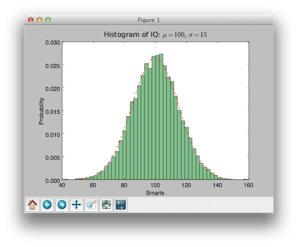
I think it's very cute!

is a command shell for interactive computing in several programming languages, originally developed for the programming language Python. allows you to expand the presentation capabilities, adds shell syntax, autocompletion and an extensive command history. currently provides the following features:

• Powerful interactive shells (terminal type and based on Qt).
• Browser-based editor with support for code, text, math expressions, embedded graphs, and other presentation capabilities.
• Supports interactive data visualization and use of GUI tools.
• Flexible, built-in interpreters for working in your own projects.
• Easy-to-use, high-performance parallel computing tools.

IPython website:

To install IPython on Linux, run the following commands in the terminal:

sudo apt-get update sudo pip install ipython

I will give an example of code that builds linear regression for a certain set of data available in the package scikit-learn:

import matplotlib.pyplot as plt import numpy as np from sklearn import datasets, linear_model # Load the diabetes dataset diabetes = datasets.load_diabetes() # Use only one feature diabetes_X = diabetes.data[:, np.newaxis] diabetes_X_temp = diabetes_X[: , :, 2] # Split the data into training/testing sets diabetes_X_train = diabetes_X_temp[:-20] diabetes_X_test = diabetes_X_temp[-20:] # Split the targets into training/testing sets diabetes_y_train = diabetes.target[:-20] diabetes_y_test = diabetes.target[-20:] # Create linear regression object regr = linear_model.LinearRegression() # Train the model using the training sets regr.fit(diabetes_X_train, diabetes_y_train) # The coefficients print("Coefficients: \n", regr .coef_) # The mean square error print("Residual sum of squares: %.2f" % np.mean((regr.predict(diabetes_X_test) - diabetes_y_test) ** 2)) # Explained variance score: 1 is perfect prediction print ("Variance score: %.2f" % regr.score(diabetes_X_test, diabetes_y_test)) # Plot outputs plt.scatter(diabetes_X_test, diabetes_y_test, color="black") plt.plot(diabetes_X_test, regr.predict(diabetes_X_test), color ="blue", linewidth=3) plt.xticks()) plt.yticks()) plt.show()

import matplotlib. pyplot as plt import numpy as np from sklearn import datasets , linear_model # Load the diabetes dataset diabetes=datasets. load_diabetes() # Use only one feature diabetes_X = diabetes . data [ : , np . newaxis ]

|

Machine learning is the study of computer science, artificial intelligence, and statistics. The focus of machine learning is training algorithms to learn patterns and make predictions in data. Machine learning is especially valuable because it allows us to use computers to automate decision-making processes.

There are so many applications for machine learning now. Netflix and Amazon use machine learning to display new recommendations. Banks use it to detect fraudulent activity in transactions with credit cards, and healthcare companies are beginning to use machine learning to monitor, assess and diagnose patients.

This tutorial will help you implement a simple machine learning algorithm in Python using the Scikit-learn tool. To do this, we will use a breast cancer database and a Naive Bayes (NB) classifier, which predicts whether a tumor is malignant or benign.

Requirements

To get started, you will need a local Python 3 development environment and a pre-installed Jupyter Notebook application. This application is very useful when running machine learning experiments: it allows you to run short blocks of code and quickly view the results, easily test and debug your code.

The following manuals will help you set up such an environment:

1: Import Scikit-learn

First you need to install the Scikit-learn module. It is one of the best and most documented Python libraries for machine learning.

To get started with your project, deploy the Python 3 development environment. Make sure you are in the directory where the environment is stored and run the following command:

My_env/bin/activate

After that, check if the Sckikit-learn module has been installed previously.

python -c "import sklearn"

If the sklearn module is installed, the command will execute without errors. If the module is not installed, you will see an error:

Traceback (most recent call last): File " ", line 1, in ImportError: No module named "sklearn"

To download the library, use pip:

pip install scikit-learn

Once the installation is complete, launch Jupyter Notebook:

jupyter notebook

In Jupyter, create an ML Tutorial document. In the first cell of the document, import the sklearn module.

Now you can start working with the dataset for your machine learning model.

2: Importing datasets

This guide uses the Wisconsin Breast Cancer Diagnostic Database. The data set includes various information about breast cancer, as well as classification labels (malignant or benign tumors). The dataset consists of 569 instances and 30 attributes (tumor radius, texture, smoothness, area, etc.).

Based on this data, a machine learning model can be built that can predict whether a tumor is malignant or benign.

Scikit-learn comes with several datasets, including this one. Import and download the dataset. To do this, add to the document:

...
from sklearn.datasets import load_breast_cancer
# Load dataset
data = load_breast_cancer()

The data variable contains a dictionary whose important keys are the names of classification labels (target_names), labels (target), attribute names (feature_names) and attributes (data).

Import the GaussianNB module. Initialize the model using the GaussianNB() function, and then train the model by fitting it to the data using gnb.fit():

...

# Initialize our classifier
gnb = GaussianNB()
# Train our classifier

You can then use the trained model to make predictions on a test dataset, which is used using the predict() function. The predict() function returns an array of predicted results for each data instance in the test set. All predictions can then be displayed.

Use the predict() function on the test set and display the result:

...
# Make predictions
preds = gnb.predict(test)
print(preds)

Run the code.

In the Jupyter Notebook output, you will see that the predict() function returns an array of 0s and 1s that represent the program's predicted results.

5: Model accuracy assessment

Using an array of class labels, you can evaluate the accuracy of the model's predicted values ​​by comparing two arrays (test_labels and preds). To determine the accuracy of a machine learning classifier, you can use the accuracy_score() function.

...

# Evaluate accuracy

Based on the results, this NB classifier has an accuracy of 94.15%. This means that he assesses 94.15% of situations correctly and can predict the outcome.

You've created your first machine learning classifier. Now we need to reorganize the code by moving all import statements to the beginning of the document. The resulting code should look like this:

from sklearn.datasets import load_breast_cancer
from sklearn.model_selection import train_test_split
from sklearn.naive_bayes import GaussianNB
from sklearn.metrics import accuracy_score
# Load dataset
data = load_breast_cancer()
# Organize our data
label_names = data["target_names"]
labels = data["target"]
feature_names = data["feature_names"]
features = data["data"]
# Look at our data
print(label_names)
print("Class label = ", labels)
print(feature_names)
print(features)
# Split our data
train, test, train_labels, test_labels = train_test_split(features,
labels,
test_size=0.33,
random_state=42)
# Initialize our classifier
gnb = GaussianNB()
# Train our classifier
model = gnb.fit(train, train_labels)
# Make predictions
preds = gnb.predict(test)
print(preds)
# Evaluate accuracy
print(accuracy_score(test_labels, preds))

Now you can continue working with this code and add more complexity to your classifier. You can experiment with different subsets of functions or try other algorithms. More machine learning ideas can be found at