Automatic rounding in excel. How to round up and down in Excel

- This working programm, included in the package Microsoft Office. It is in wide demand because it is used for various mathematical calculations, drawing diagrams, creating tables, etc. Today's topic of conversation is rounding numerical values in a program in order to obtain either the fractional part or the exact part. Using this function, answers to the following questions will be considered:

1. How can you round a number in Excel?
2. What formula is used to activate the function?
3. How do I round up or down?

Different rounding methods

When working with numerical data in Excel, sometimes it is necessary to round the calculation results to the required number of decimal places after division. The program has such an opportunity. Let's look at how you can do this in several ways:

1. Rounding the value in the cell, but not the number. This method does not affect the calculation result, but significantly improves the perception of the derived values ​​in Excel document. To do this, you should highlight required cells and use the command in the “Home” menu - “Number”, where the options for decreasing/increasing the bit depth will be presented.
2. You can also round by using the “Format Cells” button and going to the corresponding icon in the “Number” field. Click here right click mouse onto the painted cells, after which it will open desired window. In the menu you can select the number of decimal places, that is, the number of values ​​after the decimal point. The procedure itself through formatting in Excel is carried out according to the usual mathematical abbreviation.
3. can also help achieve desired result. Rounding in this way is carried out by using the “Formulas” command in the “Function Library” field, where you should select “Mathematical”.

ABOUT the latter method Let's talk in more detail.

How to use formulas?

IN open document create the right size table and fill it out. From the cell with the numbers that need to be correctly abbreviated, click on the empty cell, and then place the cursor on the line “Fx” and click on the corresponding icon. In this line we put the “=” sign and the word “ROUND”, after which in parentheses we put the address of the location of the desired cell, for example B4, and separated by a semicolon a number indicating the required number of decimal places to which the data needs to be rounded. It will turn out something like this: = ROUND(B4,1). We activate the formula by pressing the “Enter” key.

If you want to round to the nearest whole number, you must enter a 0 after the semicolon, and enter a negative number to the nearest multiple of 10.

You can also use the above formula to make a reduction to the nearest number that is a multiple of the given figure. To do this, select and click on the cell with the 1st formula, then drag the small square located in the lower right corner down. This will copy the specified formula to other cells.

When working with numbers in Excel, you often need to round a number. In most cases, the number is rounded to hundredths, tenths, or to the nearest whole number. Sometimes there are more rare cases when you need to round a number to the nearest multiple.

But whatever rounding method you need, it can be implemented in Excel. In this article we will look at 2 main ways of rounding, using cell formatting and using formulas. Excel 2010 will be used as an example, but the article will also be relevant for Excel users 2007, 2013 and 2016.

If you need to round a number that is displayed in a cell, but do not need to change the number itself that is in that cell, then rounding using cell formatting is suitable for you.

This is done very simply, select the cells with the mouse, the numbers in which you want to round, and go to the “Home” tab. Here, in the settings block called “Number”, there will be two buttons: “Increase bit depth” and “Decrease bit depth”. The first button increases the number of decimal characters that are displayed in the cell, and the second button correspondingly decreases the number of characters displayed.

A similar action can be done by right-clicking on the cell whose value you want to round and go to “Format Cells”.

In the “Format Cells” window, you need to select the number format of the cell, after which you can specify to what decimal place you want to round the number.

As you can see this method Rounding numbers is very simple. But, you need to remember that in in this case Only the number displayed in the cell is rounded, while the number actually stored in the cell remains unrounded. If you need to round a number stored in a cell, then you need to use formulas to do this. Next we will consider just this method of rounding.

Round a number using a formula

To round numbers in Excel, there are the following formulas:

• ROUND – Rounds to the nearest value. If you use this formula and round to a whole number, then 1.5 will be rounded to 2, and 1.4 to 1.
• ROUNDUP—Rounds up. If you use this formula and round to the nearest whole number, then both 1.5 and 1.4 will be rounded to 2.
• ROUND DOWN—Rounds down. If you use this formula and round to a whole number, then both 1.5 and 1.4 will be rounded to 1.
• ROUND – Performs rounding to the target multiple. Using this formula, you can round a number so that it becomes a multiple of a given number.

Using these formulas is quite simple. To do this, you need to select the cell in which the rounded number should be located and select this cell with the mouse. After this, you need to enter the formula in this cell as follows:

• First you need to write an equal sign (=) and the name of the formula (for example, ROUND).
• Next, open the parenthesis and indicate the address of the cell whose value needs to be rounded (for example, G3).
• Next we put a semicolon (;).
• Next, enter the number of decimal places you want to get after rounding. If you need to round to a whole number, enter 0.
• After that, close the parenthesis and press Enter to save the typed formula.

If everything was done correctly, a rounded number will appear in the cell you selected. If you made mistakes when entering the formula, Excel will notify you about this using a pop-up window.

The screenshot above shows the process of typing the formula. This formula involves rounding the number in cell G3 and placing the result in cell H3.

How to round a number to a whole number in Excel

We will separately consider rounding to a whole number, since this problem occurs most often. In order to round the existing number to a whole number, you can use the formulas ROUND, ROUNDUP or ROUND DOWN. If you simply need to round a number to the nearest whole number, use the ROUND formula. To round to a larger integer, use ROUNDUP, and to round to a smaller integer, ROUNDDOWN.

For clarity, let's look at the whole process step by step. Select the cell where the rounded number should be located and select it with the mouse.

Enter the cell address of the number you want to round to the nearest whole number (in this case, cell G3) and insert a semicolon (;).

As a result, in cell H3 you will receive the number from cell G3, but rounded to the nearest whole value.

If you need to change the number of zeros after the decimal point displayed, this can be done using formatting, as described at the beginning of the article.

Program Microsoft Excel It also works with numerical data. When performing division or working with fractional numbers, the program performs rounding. This is due, first of all, to the fact that absolutely accurate fractional numbers are rarely needed, but operating with a cumbersome expression with several decimal places is not very convenient. In addition, there are numbers that, in principle, cannot be rounded accurately. But, at the same time, insufficiently accurate rounding can lead to gross mistakes in situations where precision is required. Fortunately, Microsoft Excel allows users to set how numbers will be rounded.

All the numbers it works with Microsoft program Excel are divided into exact and approximate. Numbers up to the 15th digit are stored in memory, and are displayed up to the digit specified by the user. But, at the same time, all calculations are performed according to the data stored in memory, and not displayed on the monitor.

Using the rounding operation, Microsoft Excel discards a certain number of decimal places. Used in Excel generally accepted method rounding, when a number less than 5 is rounded down, and greater than or equal to 5 is rounded up.

Rounding using ribbon buttons

The most in a simple way To change the rounding of a number is to select a cell or group of cells, and being in the “Home” tab, click on the “Increase bit depth” or “Decrease bit depth” button on the ribbon. Both buttons are located in the “Number” tool block. In this case, only the displayed number will be rounded, but for calculations, if necessary, up to 15 digits of numbers will be used.

When you click on the “Increase decimal place” button, the number of decimal places entered increases by one.

When you click the “Decrease decimal place” button, the number of digits after the decimal point is reduced by one.

Rounding via cell format

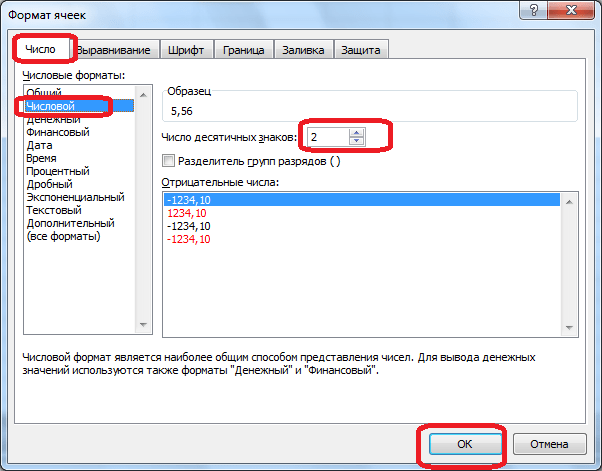
You can also set rounding using the cell format settings. To do this, you need to select a range of cells on the sheet, right-click, and select “Format Cells” in the menu that appears.

In the cell format settings window that opens, go to the “Number” tab. If the data format specified is not numeric, then you must select a numeric format, otherwise you will not be able to adjust rounding. In the central part of the window, near the inscription “Number of decimal places,” we simply indicate with a number the number of digits that we want to see when rounding. After this, click on the “OK” button.

Setting the accuracy of calculations

If in previous cases, the parameters set affected only the external display of data, and more accurate indicators were used in the calculations (up to the 15th digit), now we will tell you how to change the accuracy of the calculations.

A window opens Excel settings. In this window, go to the “Advanced” subsection. We are looking for a settings block called “When recalculating this book”. The settings in this section apply not to a single sheet, but to the entire workbook as a whole, that is, to the entire file. Check the box next to the “Set accuracy as on screen” option. Click on the “OK” button located in the lower left corner of the window.

Now, when calculating data, the displayed value of the number on the screen will be taken into account, and not the one stored in Excel's memory. The displayed number can be configured in any of the two ways that we discussed above.

Applying functions

If you want to change the rounding amount when calculating relative to one or more cells, but do not want to reduce the accuracy of calculations as a whole for the document, then in this case, it is best to take advantage of the opportunities provided by the “ROUND” function and its various variations, as well as some other functions.

Among the main functions that regulate rounding are the following:

• ROUND – rounds to the specified number of decimal places, according to generally accepted rounding rules;
• ROUNDUP – rounds up to the nearest number;
• ROUNDDOWN – rounds down to the nearest number;
• ROUND – rounds a number from specified accuracy Yu;
• OKRVERCH – rounds a number with a given accuracy up to the absolute value;
• OKRVNIZ – rounds a number down modulo with a specified accuracy;
• OTBR – rounds data to a whole number;
• EVEN – rounds data to the nearest even number;
• ODD – Rounds data to the nearest odd number.

For the ROUND, ROUNDUP and ROUNDDOWN functions, the following input format is: “Function name (number; number_digits). That is, if you, for example, want to round the number 2.56896 to three digits, then use the ROUND(2.56896;3) function. The output is 2.569.

For the functions ROUNDUP, OKRUP and OKRBOTTEN, the following rounding formula is used: “Name of function (number, precision)”. For example, to round the number 11 to the nearest multiple of 2, enter the function ROUND(11;2). The output is the number 12.

The functions DISRUN, EVEN and ODD use the following format: “Function name (number)”. To round the number 17 to the nearest even number, use the EVEN(17) function. We get the number 18.

A function can be entered both in a cell and in the function line, having previously selected the cell in which it will be located. Each function must be preceded by an “=” sign.

There is a slightly different way to introduce rounding functions. It is especially useful when you have a table with values ​​that need to be converted to rounded numbers in a separate column.

To do this, go to the “Formulas” tab. Click on the “Mathematics” button. Next, in the list that opens, select the desired function, for example ROUND.

After this, the function arguments window opens. In the “Number” field, you can enter a number manually, but if we want to automatically round the data of the entire table, then click on the button to the right of the data entry window.

The function arguments window is minimized. Now you need to click on the topmost cell of the column whose data we are going to round. After the value is entered into the window, click on the button to the right of this value.

The function arguments window opens again. In the “Number of digits” field, write down the digit number to which we need to reduce the fractions. After this, click on the “OK” button.

As you can see, the number has been rounded. In order to round all other data in the desired column in the same way, move the cursor over the lower right corner of the cell with the rounded value, click on left button mouse and drag it down to the end of the table.

After this, all values ​​in required column will be rounded.

As you can see, there are two main ways to round the visible display of a number: using a button on the ribbon, and by changing the cell format parameters. In addition, you can change the rounding of the actual calculated data. This can also be done in two ways: by changing the settings of the book as a whole, or by using special functions. Choice specific method depends on whether you are going to apply this type of rounding to all data in the file, or only to certain range cells.

In this article we will look at one of the office applications MS Office Excel.

MS Office Excel is a program that is part of the Microsoft Office suite. Used for various mathematical calculations, drawing diagrams, creating tables, etc.

The program document is workbook. The book consists of an unlimited number of sheets, set by the user.

Each sheet of the program is a table consisting of 65536 rows and 256 columns. Each cell of such a table is called a cell.

An Excel cell has its own individual address, consisting of a row and column number (for example, 1A, 2B, 5C).

Main functions of the program

Function "SUM" (sum in Excel)

There are three methods for summing digits and numbers in Excel.

1. Using the standard addition sign - plus (“+”). Most often, this method is used when adding a small number of digits or numbers, as well as inside formulas for adding calculations of other functions.
2. Using the "SUM" function input and selecting arguments. Allows you to add numbers located in a single array (part of a column, row), several non-adjacent cells, one two-dimensional array, an array adjacent cells and non-adjacent parts. Any amount can be calculated in Excel using this function.
3. Using the autosum symbol "Σ" and selecting a range of terms. Used to calculate the amount in the same cases as "SUM".

Formula "ROUND"

The result of any calculation, just like the sum in Excel, can be displayed in Excel; it is important not to confuse it with displaying the value.
To perform the “rounding in Excel” action, you must select the cell containing the calculation result, put an equal sign (“=”) in front of the number, select the “ROUND” function and set the required number of digits.

Regarding the display of characters, it should be noted that the cell displays the number of digits that are placed in it for user visibility. But in this case, rounding as such does not occur. When the cell size changes, the number of digits also changes both upward, as the cell increases, and downwards, when it decreases.

As you can see, rounding in Excel is not such a difficult task.

"PROPNACH", "DLstr"- text functions that allow you to change the length of a line or the case used, as well as combine or split lines.

"BDCOUNT", "BDSUMM"- functions for databases. Allows you to count the number of database records and the sum of values. These functions are similar to the sum function in Excel of the “SUM” type.

"CELL"- this function provides the user with information about the properties of the cell.

Mathematical functions- Excel core. Calculations using them are the main purpose of the program. Excel has a huge variety of mathematical functions, such as arccosine, arcsine, tangent, cotangent. When using these functions, multi-digit values ​​are often obtained. So the “Rounding in Excel” section of this article will come in handy in this case as well.

"MUMNOUZH", "MOPRED", "MOBR" for operations with numeric arrays and matrices.

"UNIT", "INTERMEDIATE" to obtain final and intermediate values.

Logarithms, linear logarithms, decimal logarithms.

Statistical. "BETAOBR"- returns to the integral beta probability density function. "WEIBULL"- return of the Weibull distribution.

Also MS Office Excel has financial functions, functions links and arrays, functions dates and times, checking assignments and properties.

So this program is an indispensable assistant for people of any professions who are in one way or another connected with numbers and figures.

Rounding in Excel is primarily necessary for convenient formatting of numbers.

This can be done either up to an integer value or up to a certain number of decimal places.

Round a number to a certain number of decimal places

It is worth noting that numbers must be rounded correctly. It's not enough to simply remove a few decimal places from a long value.

Otherwise, the final calculations in the document will not converge.

You can round using the built-in functionality of the program. In fact, the number is updated only visually, and the real value of the number remains in the cell.

In this way, calculations can be carried out without data loss, while the user will be comfortable working with large sums and prepare the final report.

The figure shows a list of the main rounding functions and the result of their use:

To commit simple procedure rounding numbers to several decimal places (in this case, up to 2 decimal places), follow the instructions:

• Open a previously used document or create a new one and fill it with the necessary data;
• In the tab for working with formulas, open the drop-down list with mathematical functions and find those that are intended for rounding, as shown in the figure below;

• Enter the function arguments and fill in all fields of the dialog box as shown in the figure;

• The resulting function will be written in the cell's formula field. To apply it to all other cells, copy it.

Rounding to a whole number

To round up decimal number to the whole, you can use several functions at once, namely:

• OKRVVERH– using this function, you will be able to round up to an integer value.
• ROUND– rounds the selected number according to all canons of mathematical rules;
• OKRVNIZ is a function that is designed to round a decimal to an integer value down from the integer.
• OTBR– the function discards all digits after the decimal point, leaving only the integer value;
• CHETN– rounding to an integer value until the result is even;
• ODD- function opposite to EVEN;
• ROUND– rounding with the accuracy specified by the user in the program dialog box.

Using the above functions, you can create an integer number as per the user's requirement.

After selecting the function, in the dialog box that opens, specify the precision equal to zero.

Thus, decimal places will not be taken into account.