How to make a selection from a list in excel. Creating a Dropdown List in Excel
Users who quite often work in Excel and maintain their databases in this program probably often need to select a cell value from a predetermined list.
For example, we have a list of product names, and our task is to fill each cell of a certain table column using this list. To do this, you need to create a list of all items, and then implement the ability to select them in the required cells. This solution will eliminate the need to write (copy) the same name manually many times, and will also save you from typos and other possible errors, especially when it comes to large tables.
You can implement the so-called drop-down list using several methods, which we will consider below.
The simplest and most understandable method is to first create a list elsewhere in the document. You can place it next to the table, or create a new sheet and make a list there, so as not to “clutter” the original document with unnecessary elements and data.
- In the auxiliary table we write a list of all names - each on a new line in a separate cell. The result should be one column with filled data.
- Then we mark all these cells, right-click anywhere in the marked range and in the list that opens, click on the “Assign a name..” function.

- The “Create a name” window will appear on the screen. We name the list whatever we want, but with the condition that the first character must be a letter, and the use of certain characters is not allowed. It also allows you to add a note to the list in the corresponding text field. When ready, click OK.

- Switch to the “Data” tab in the main program window. We mark the group of cells for which we want to set a selection from our list and click on the “Data Validation” icon in the “Working with Data” subsection.

- The “Checking entered values” window will appear on the screen. While in the “Parameters” tab, in the data type, select the “List” option. In the “Source” text field, write the equal sign (“=”) and the name of the newly created list. In our case – “=Name”. Click OK.

- Everything is ready. To the right of each cell of the selected range, a small icon with a down arrow will appear, by clicking on which you can open the list of items that we have compiled in advance. By clicking on the desired option from the list, it will immediately be inserted into the cell. In addition, the value in a cell can now only correspond to the name from the list, which will eliminate any possible typos.

You can create a drop-down list in another way - through developer tools using ActiveX technology. The method is somewhat more complicated than described above, but it offers a wider range of tools for customizing the list: you can set the number of elements, the size and appearance of the list box itself, the need to match a value in a cell with one of the list values, and much more.
- First of all, these tools need to be found and activated, since they are turned off by default. Go to the “File” menu.

- In the list on the left, find the “Options” item at the very bottom and click on it.

- Go to the “Customize Ribbon” section and in the “Main Tabs” area, check the box next to “Developer”. Developer tools will be added to the program ribbon. Click OK to save the settings.

- The program now has a new tab called “Developer”. We will work through it. First, we create a column with elements that will be the sources of values for our drop-down list.

- Switch to the “Developer” tab. In the “Controls” subsection, click on the “Insert” button. In the list that opens, in the “ActiveX Controls” function block, click on the “Combo Box” icon.

- Next, click on the desired cell, after which a list window will appear. We adjust its dimensions along the cell boundaries. If the list is selected with the mouse, “Design Mode” will be active on the toolbar. Click on the “Properties” button to continue setting up the list.

- In the parameters that open, find the line “ListFillRange”. In the column next to us, separated by a colon, we write the coordinates of the range of cells that make up our previously created list. Close the window with parameters by clicking on the cross.

- Then right-click on the list window, then click on the “ComboBox Object” item and select “Edit”.

- As a result, we get a drop-down list with a predefined list.

- To insert it into several cells, move the cursor over the lower right corner of the cell with the list, and as soon as it changes its appearance to a cross, hold down the left mouse button and drag down to the very bottom line in which we need a similar list.

Users also have the ability to create more complex interdependent (linked) lists. This means that the list in one cell will depend on what value we have selected in another. For example, we can set kilograms or liters in product units. If you select kefir in the first cell, in the second you will be offered two options to choose from - liters or milliliters. And if in the first cell we choose apples, in the second we will have a choice of kilograms or grams.
- To do this, you need to prepare at least three columns. The first will contain the names of the goods, and the second and third will contain their possible units of measurement. There may be more columns with possible variations of units of measurement.

- First, we create one general list for all product names by selecting all the rows of the “Name” column through the context menu of the selected range.

- Give it a name, for example, “Food”.

- Then, in the same way, we create separate lists for each product with the corresponding units of measurement. For greater clarity, let’s take as an example the first position – “Bow”. We mark the cells containing all units of measurement for this product and, through the context menu, assign a name that must completely match the name.
 In the same way, we create separate lists for all other products in our list.
 - After this, we insert a general list of products into the top cell of the first column of the main table - as in the example described above, through the “Data Check” button (the “Data” tab).

- We indicate “=Nutrition” as the source (according to our name).

- Then click on the top cell of the column with units of measurement, also go to the data verification window and indicate the formula in the source “ =INDIRECT(A2)“, where A2 is the number of the cell with the corresponding product.

- The lists are ready. All that remains is to stretch them all the rows of the table, both for column A and column B.

Hello everyone, dear friends and guests of my blog. And again I am with you, Dmitry Kostin, and today I would like to tell you more about Excel, or rather about one wonderful feature that I now always use. Have you encountered the situation? when you fill out a table and in some column you need to constantly enter one of several values. Uhhh. Let me tell you better with an example.
Let’s say, when I created a computer equipment accounting table (a long time ago) at my work, in order to make the whole work process more convenient and faster, I made a drop-down list in certain columns and inserted certain values there. And when I filled out the “Operating system” column (but it’s not the same on all computers), I filled in several values (7, 8, 8.1, 10), and then simply selected it all with one click of the mouse button.
And thus, you no longer need to type the version of Windows into each cell, or copy from one cell and paste into another. In general, I won’t bore you, let’s get started. Let me show you how to create a dropdown list in excel using data from another sheet. To do this, let's create some kind of table to which we can apply this. I will do this in the 2013 version, but the process is identical for other versions, so don't worry.
Preparation

Basic steps

Now work with graphs in exactly the same way "Name of specialist" And "Result of elimination", then return to the main sheet again and start working fully with the table. You will see for yourself how cool and convenient it is when you can select data from available pre-prepared values. This makes routine filling of tables easier. 
By the way, in such documents, for more convenient display, it is better. Then everything will be cool.
Well, I’m finishing my article for today. I hope that what you learned today will be useful to you when working in Excel. If you liked the article, then of course do not forget to subscribe to my blog updates. Well, I’ll be looking forward to seeing you again on the pages of my blog. Good luck and bye-bye!
Best regards, Dmitry Kostin
In order not to type in letters and numbers the previously typed text and numeric values of cells, to speed up the process of filling out the cells of an MS Excel sheet with information and to minimize errors, including typos and spelling errors, it is convenient to use a drop-down list.
From the drop-down list, with a few clicks of the mouse, you can enter the necessary information into the designated cells. Drop-down lists are widely used when writing calculation programs in Excel.
The MS Excel program, having a very user-friendly interface, offers the user several different options for assistance when entering repeating information into worksheet cells.
Let's assume that we maintain a database of rolled metal receipts at a warehouse. In the first column we indicate the type of rolled profile.
Option #0 - “Elementary”.
 When making the next entry in cell A9, when typing the first letter of the profile name, for example “Ш”, Excel suggests filling the cell with the word “Channel”. After typing “Ш”, just press the “Enter” button on the keyboard - and the word will be entered into the cell.
The “disadvantage” of this option is the need to enter sometimes several letters and the inability to create a directory of names in advance, which limits the user’s freedom of activity.
Let's move directly to the options for creating drop-down lists.
Option #1 - “The simplest”.
 If you activate cell A9 with the mouse and press the key combination “Alt” “↓”, a drop-down list will appear containing all the values previously entered in this column. All that remains is to select the desired entry with the mouse. Instead of typing the above keyboard shortcut, you can right-click to open the context menu and select “Select from drop-down list...” from it. As a result, we will see the same drop-down list.
In this version, the active cell must be adjacent to the bottom of the range of values, and the range itself must not contain empty cells!
Option #2 - “Simple”.

This option allows you to create in advance a list (directory) of values from which the user can later select the necessary records. In this case, the list can be placed anywhere on the sheet (or even on another sheet) and can be hidden from the user if necessary.
In order to create a drop-down list in this option, you need to follow a series of sequential steps.
1. We create a list of possible values by writing them into a column, one per cell. Let's say this is a list in cells A2...A8.
2. We activate the cell in which we want to place the drop-down list by placing the cursor in it. Let this be the same cell A9.
3. In the main menu, select the “Data” – “Check...” button.
4. In the “Checking entered values” window that pops up, select the “Parameters” tab.
5. In the “Data type:” field, from the drop-down list (similar to the one we are creating), select the “List” value.
6. In the “Source:” field that appears, specify a range containing a list of possible values.
7. Check (if it is not checked by default) the “List of valid values” checkbox and click the “OK” button.

The dropdown list is ready. It can be copied as formulas into any number of cells!
Option #3 - “Complicated”.

This option for creating a drop-down list, despite its name “Complex,” is essentially not that. To create a drop-down list, it uses the Combo Box item on the Forms toolbar.
Let's create a drop-down list using this method.
1. We create a reference list in cells A2...A8.
2. In the main menu, select the button “View” – “Toolbars” – “Forms”.
3. In the “Forms” panel that appears, select “Combo Box” and draw it, for example, in cell A9.
The “Combo Box” element is placed not in the cell itself, but, as it were, above it!!! The element can be large and over several cells.
4. Right-click on the drawn element and select “Format Object” in the context menu that appears.
5. In the “Object Formatting” window that pops up, on the “Control” tab, fill in the fields in accordance with the figure below and click “OK”.

6. The dropdown list is ready. It outputs the sequence number of the list item in the associated cell B9. (You can assign any cell convenient for you, not necessarily B9!)
To display the value itself from the reference list in any cell, use the INDEX function. Let's say we need to display a value in cell A9, located under the “Combo Box” element.
To do this, write the formula in cell A9: =INDEX(A2:A8,B9)
A clear example is discussed in detail in the article “”. You can follow the link and check it out.
The drop-down list created in this way plus the use of the INDEX and/or VLOOKUP functions provide limitless possibilities for the user when retrieving data from various underlying lookup tables.
Option number 4 - “The most difficult”.
 To create a drop-down list in this case, the “Combo Box” element is also used, but the “Controls” toolbar (in MS Excel 2003). These are so-called ActiveX controls. Here everything is very similar in appearance to option No. 3, but the possibilities for customizing and formatting the element are much wider.
1. In the main menu, select the button “View” – “Toolbars” – “Controls”.
2. In the “Controls” panel that appears, select “Combo Box” and draw it in cell A9. ElementActiveXThe “combo box” is not placed in the cell itself, but on top, covering it!!!
 3.
Click the “Properties” button on the “Controls” panel and in the “Properties” window that pops up, manually enter the range of source data, the address of the associated cell (the cell where the selected value will be entered) and the number of displayed rows.
3.
Click the “Properties” button on the “Controls” panel and in the “Properties” window that pops up, manually enter the range of source data, the address of the associated cell (the cell where the selected value will be entered) and the number of displayed rows.
4. Then, if you wish, you can change the font, its color, background color, and a number of other parameters... There is nothing complicated in using the “Most Difficult” option - see for yourself. Everything is intuitive, although basic knowledge of English will not hurt!
5. Press the “Exit Design Mode” button on the “Controls” panel and check the operation of the drop-down list. Everything works! The selected value is written in cell A9, in our example - under the “Combo Box” element. In general, a linked cell can be absolutely any cell except the cells where the base list is located.
Results.
Option No. 0 automates the filling of cells to some extent, but, of course, has nothing to do with drop-down lists and is given here under the corresponding number as an elementary option for automating the entry of repeating data.
In practice, I most often create drop-down lists in Excel using options No. 1 and No. 3, less often - option No. 2, and very rarely - option No. 4, although it is by far the most flexible and provides the widest possibilities.
But often our choices in life are determined by tastes, stereotypes and habits! Depending on the task that needs to be solved when working in Excel, you should choose the most appropriate and convenient option for creating drop-down lists for each specific case.
Subscribe to article announcements in the window located at the end of each article or in the window at the top of the page and don't forget to confirm subscribe by clicking on the link in the letter that will be sent to you at the specified email address (it may arrive in the Spam folder - it all depends on your email settings)!!!
Was this article useful or not for you, dear readers? Write about it in the comments.
A drop-down list refers to the content of several values in one cell. When the user clicks on the arrow on the right, a specific list appears. You can choose a specific one.
A very convenient Excel tool for checking entered data. The capabilities of drop-down lists allow you to increase the comfort of working with data: data substitution, display of data from another sheet or file, the presence of a search function and dependencies.
Creating a Dropdown List
Path: Data menu - Data Validation tool - Options tab. Data type – “List”.
You can enter the values from which the drop-down list will be composed in different ways:

Any of the options will give the same result.
Dropdown list in Excel with data substitution
You need to make a drop-down list with values from the dynamic range. If changes are made to the existing range (data is added or removed), they are automatically reflected in the drop-down list.

Let's test it. Here is our table with the list on one sheet:

Let’s add a new value “Christmas tree” to the table.

Now let’s remove the “birch” value.

The “smart table”, which easily “expands” and changes, helped us realize our plans.
Now let's make it possible to enter new values directly into the cell with this list. And the data was automatically added to the range.


When we enter a new name into an empty cell of the drop-down list, a message will appear: “Add the entered name baobab to the drop-down list?”
Click “Yes” and add another line with the value “baobab”.
Dropdown list in Excel with data from another sheet/file
When the values for the dropdown list are located on another sheet or in another workbook, the standard method does not work. You can solve the problem using the INDIRECT function: it will generate the correct link to an external source of information.
- We make active the cell where we want to place the drop-down list.
- Open data verification options. In the “Source” field, enter the formula: =INDIRECT(“[List1.xlsx]Sheet1!$A$1:$A$9”).
The name of the file from which the information for the list is taken is enclosed in square brackets. This file must be open. If the book with the required values is located in another folder, you need to specify the full path.
How to make dependent dropdown lists
Let's take three named ranges:

This is a must. The above describes how to make a regular list a named range (using the “Name Manager”). Remember that the name cannot contain spaces or punctuation marks.
- Let's create the first drop-down list, which will include the names of the ranges.
- When you have placed the cursor in the “Source” field, go to the sheet and select the required cells one by one.
- Now let's create a second dropdown list. It should reflect those words that correspond to the name selected in the first list. If “Trees”, then “hornbeam”, “oak”, etc. Enter in the “Source” field a function of the form =INDIRECT(E3). E3 – cell with the name of the first range.
- We create a standard list using the Data Validation tool. We add a ready-made macro to the source code of the sheet. How to do this is described above. With its help, the selected values will be added to the right of the drop-down list. Private Sub Worksheet_Change(ByVal Target As Range) On Error Resume Next If Not Intersect(Target, Range("E2:E9")) Is Nothing And Target.Cells.Count = 1 Then Application.EnableEvents = False If Len(Target.Offset (0, 1)) = 0 Then Target.Offset(0, 1) = Target Else Target.End (xlToRight).Offset(0, 1) = Target End If Target.ClearContents Application.EnableEvents = True End If End Sub
- To make the selected values appear below, we insert another handler code. Private Sub Worksheet_Change(ByVal Target As Range) On Error Resume Next If Not Intersect(Target, Range("H2:K2")) Is Nothing And Target.Cells.Count = 1 Then Application.EnableEvents = False If Len(Target.Offset (1, 0)) = 0 Then Target.Offset(1, 0) = Target Else Target.End (xlDown).Offset(1, 0) = Target End If Target.ClearContents Application.EnableEvents = True End If End Sub
- To display the selected values in one cell, separated by any punctuation mark, use the following module.


Selecting multiple values from an Excel dropdown list
It happens when you need to select several items from a drop-down list at once. Let's consider ways to implement the task.
Private Sub Worksheet_Change(ByVal Target As Range)
On Error Resume Next
If Not Intersect(Target, Range("C2:C5")) Is Nothing And Target.Cells.Count = 1 Then
Application.EnableEvents = False
newVal = Target
Application.Undo
oldval = Target
If Len(oldval)<>0 And oldval<>newValThen
Target = Target & "," & newVal
Else
Target = newVal
End If
If Len(newVal) = 0 Then Target.ClearContents
Application.EnableEvents = True
End If
End Sub
Don’t forget to change the ranges to “your own”. We create lists in the classic way. And macros will do the rest of the work.
Dropdown list with search

When you enter the first letters on the keyboard, matching elements are highlighted. And these are not all the pleasant aspects of this tool. Here you can customize the visual presentation of information and specify two columns as a source at once.
There are several ways to create a dropdown list. The choice of one depends on the structure of the data you have.
The first way to create a two-level list
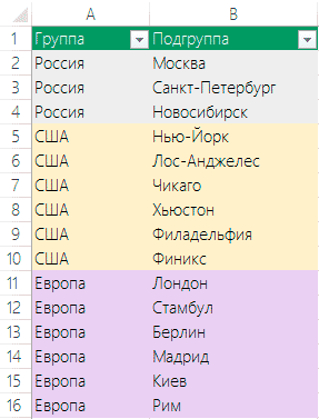
The first method is based on creating a “smart” table, the header of which contains the values of the first drop-down list (group), and the table rows correspond to the values of the second drop-down list (subgroup). The values of the subgroup elements should be located in the corresponding group column, as in the figure below.

Now let's start creating the first drop-down list of the group (in my case, a list of countries):
- Select the cell into which you will insert the drop-down list;
- Go to the ribbon tab Data;
- Choosing a team Data verification;
- Select a value from the drop-down list List;
- In the field Source indicate the following formula =INDIRECT("Table1[#Headers]").
Formula INDIRECT returns a reference to the range of smart table headers. The advantage of using such a table is that as you add columns, the dropdown list will automatically expand.
It remains to create a second dependent drop-down list - a list of subgroups.
We boldly repeat the first 4 points described above. Source in the window Data verification for the second drop-down list the formula will be =INDIRECT("Table1["&F2&"]"). Cell F2 in this case, the value of the first drop-down list.
You can also use a regular dumb table, but in this case you will have to manually change the header and row ranges. In the example considered, this happens automatically.
The second way to create a two-level list
The second method is convenient to use when the drop-down list data is written in two columns. The first contains the name of the group, and the second contains the name of the subgroup.
IMPORTANT! Before creating a dependent list by subgroups, you need to sort the source table by the first column (the column with the group); then it will be clear why this is being done.
To create a group dropdown, we need an additional column containing the unique group values from the source table. To create this list, use the Remove Duplicates feature or use the Unique command from the VBA-Excel add-in.
Now let's create a drop-down list of groups. To do this, follow the first 4 points from the first method of creating a two-level list. As Source specify a range of unique group values. Everything is standard here.
Recommendation: It is convenient to specify a named range as a source. To create it, open Name Manager from tab Formulas and give a name to the range with unique values.
Now the hardest part is to specify in Source a dynamic link to a range with the values of the second drop-down list (list of subgroups). We will solve it using the function OFFSET(link, row_offset, column_offset, [height], [width]), which returns a reference to a range that is a specified number of rows and columns away from a cell or range of cells.
- Link in our case - $A$1- upper left corner of the source table;
- Offset_by_rows - MATCH(F3,$A$1:$A$67,0)-1- line number with the value of the desired group (in my case, country cell F3) minus one;
- Offset_by_columns - 1 - since we need a column with subgroups (cities);
- [Height] - COUNTIF($A$1:$A$67,F3)- number of subgroups in the desired group (number of cities in the country F3);
- [Width] - 1 - since this is the width of our column with subgroups.